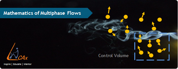
Multiphase Flow Modeling : Part 4 - Mathematical treatment
After a thematic representation about the different modeling approached of multiphase flows in Multiphase Flow Modeling using CFD, we shall now have a look at the mathematical treatments involved behind all these models viz., Eulerian-Lagrangian, Eulerian-Eulerian and Volume of fluid.
Prerequisite : The reader is already familiar with numerical treatments of Navier-Stoke's equations.
We shall not get into every detail of the mathematical equations, however shall take note of only the important equations and their significance in modeling multiphase flows.
Eulerian-Lagrangian Approach (E-L) :
The assumptions made for the Eulerian-Lagrangian approach are as follows:
- Continuous phase modeled using Eulerian framework i.e Eulerian method.
- Equation of motion solved for dispersed phase i.e Lagrangian method.
- This approach is ideally applicable for very low volume loading or volume fraction of dispersed phase as we assume that the flow of dispersed phase does not affect the flow of continuous phase in detail.
- Volume displacement due to dispersed phase motion is ignored.
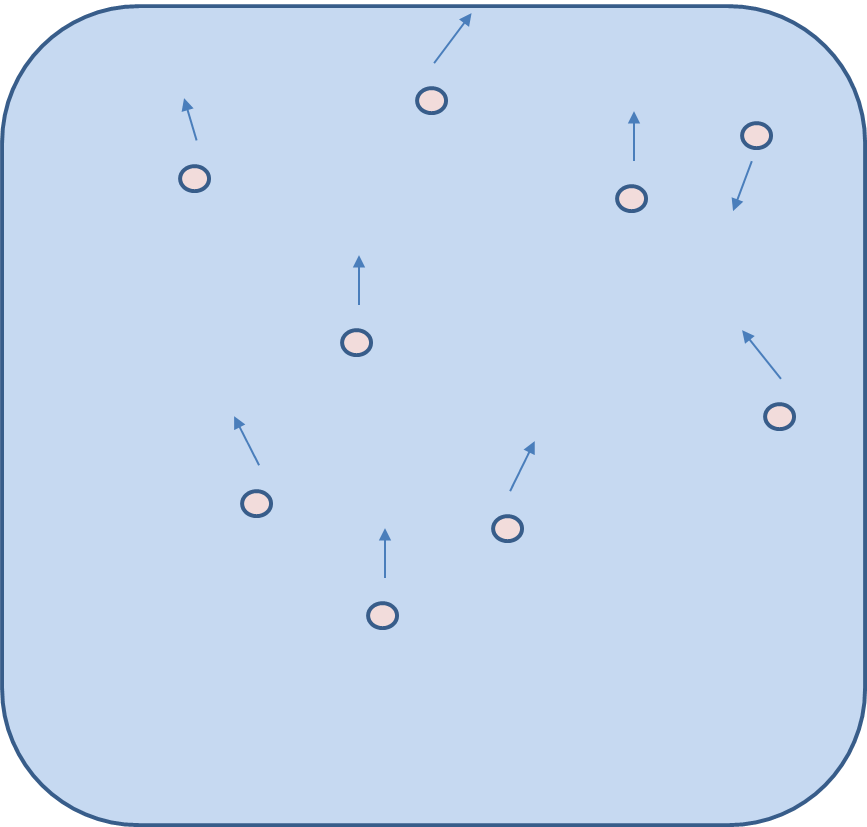
Eulerian-Lagrangian Approach
In the mathematical treatment we solve a set of continuity and momentum equations for the primary phase only and for the secondary/ dispersed phase the trajectories (of dispersed phase) are calculated by using the equation of motion. For this we use Newton's law of motion that is just a force balance taking into account the interaction between the primary and secondary phase. Below are shown the equations applied while modeling flows with the E-L approach.
Continuity equation : {tex} \frac{\partial(\alpha_c \rho_c)}{\partial t} + \nabla \cdot \alpha_c \rho_c U_c) = S_c {/tex}
Momentum equation : {tex} \frac{\partial(\alpha_c \rho_c U_c)}{\partial t} + \nabla \cdot (\alpha_c \rho_c U_c U_c) = -\alpha_c \del p - \nabla \cdot (\alpha_c T_c) + \alpha_c \rho_c g + S_{cm} {/tex}
Newton's Law of motion used for force balance of single dispersed particle:
{tex} m_P \frac{dU-P}{dt} = F_P + F_D + F_{VM} + F_L + F_H + F_G {/tex}
where: {tex} F_D {/tex} is Drag Force, {tex} F_p {/tex} is Pressure Force, {tex} F_{VM} {/tex} is Virtual Mass force, {tex} F_G {/tex} is Body Force. These individual forces are calculated by their configurations like the Pressure force is the gradient of pressure, for body force we use acceleration due to gravity and for the drag & lift force we use the relative velocities and their corresponding coefficients, also shown in the mathematical representation.
Pressure force : {tex} F_p = V_p \nabla \cdot p {/tex}
Body force due to gravity : {tex} F_G= \rho_P V_P g {/tex}
Drag force : {tex} F_D= -\frac{\pi}{8}C_D \rho_C D_{P}^{2} |{U_P - U_C}| (U_P - U_C) {/tex} where {tex} C_D \left\{ \begin{array}{l l} Re_p < 1000\Rightarrow 24/Re (1 + 0.15 Re^{0.687}) \\ Re_p <= 1000 \Rightarrow 0.44 \\ \end{array} {/tex}
{tex} Re_p= \frac{\rho C_D P |{U_P - U_C}|}{\mu_C} {/tex}
Lift force : {tex} F_L= -C_L \rho_C V_P (U_P-U_C) \times (\nabla \times U_C) {/tex}
where {tex} C_L {/tex} is the lift coefficient.
In addition to the lift and drag force there is another force also acting called as the virtual mass force. When dispersed particles accelerate some part of surrounding continuous phase fluid also accelerates with them. This extra acceleration gives an effect of added mass or inertial force in addition to the lift and drag force that gives rise to the virtual mass force, mathematically represented as below.
{tex} F_{VM}=-(\frac{Dl}{Dt} + I \nabla \cdot U_C){/tex}
So {tex}I=C_{VM} \rho_C V_P (U_P - U_C) {/tex}
Thus in E-L approach what we do is basically solve the flow equations for the primary phase then using this momentum exchange find the interactive forces between the two phases and then we calculate the velocity of the secondary phase or the dispersed particulates. Now after knowing the velocity, to find the flow path or trajectories of the dispersed phase we use the basic definition of velocity i.e.:
{tex} \frac{dx_i}{dt}= U_{pi} {/tex}
As the above equation relates velocity (U) with time derivative of location (x) we can find the path or trajectory of the secondary phase. So this is how we use the E-L approach in order to carry out modeling of dispersed phase in a 2-phase system.
Eulerian-Eulerian Approach (E-E) :
In this approach the secondary or dispersed phase is also treated as a continuum i.e the Eulerian equations are solved for both the phases. The coupling between the phases is represented by various interphase transport models. As this is a more resolved type of approach wherein we solve the set of governing equation for all the phases and the entire flow is modeled to greater accuracy hence is suitable to cases with the secondary phase as predominant i.e. for cases with volume loading more than 10%.
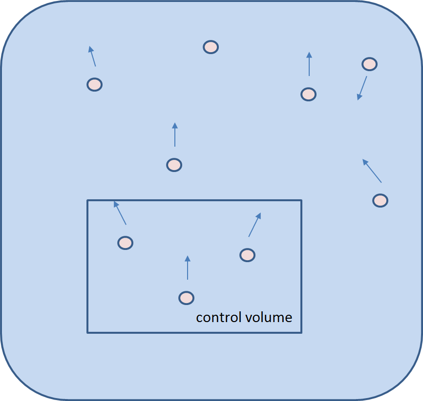
Eulerian-Eulerian Approach
Mathematical treatment of this is shown below wherein we solve the continuity and momentum equations for each phase The continuity equation for phase {tex} k {/tex} with volume fraction {tex} \alpha_k {/tex}
{tex} \frac{\partial (\alpha_k \rho_k)}{\partial t} + \nabla \cdot (\alpha_k \rho_k U_k) = \sum_{p=1, p\neq k}^{n} S_{pk} {/tex}
Also interphase coupling force balance is done for each phase: {tex} F_{kq}=-F_{qk} {/tex}
The interphase coupling terms for phase k can be written as:
{tex} \frac{\partial (\alpha_k \rho_k)}{\partial t} + \nabla \cdot (\alpha_k \rho_k U_k) = \sum_{q=1}^n Kkq(U_q - U_k) + \sum_{q=1, q\neq k} S_{qk} U_{qk} {/tex}
Volume of Fluid Approach (VOF) :
In this approach the flow around individual particles is resolved and hence we use a single set of governing equations for all the phases involved. We define here a term called as mixture properties using properties of individual phases and use it to solve the governing equations. It is suitable for stratified and separated flows where there is a distinct interphase between two or more phases.
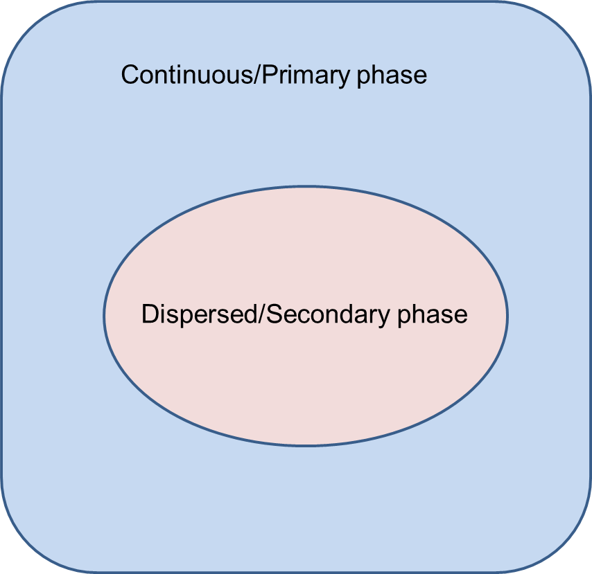
Volume of Fluid Approach
The VOF approach simulates the motion of all the phases rather than tracking the motion of interface itself. Here as we solve a single set of equation for both the phases, the tracking of interphase is not direct but needs a special treatment in order to capture it. For this we need to solve a type of advection equation for volume fraction, i.e. we basically solve a continuity equation for (n-1) phases and find out the amount of phases involved in each particular location or cell. However these advection equations are not enough as they only give the percentage amount of phase involved in particular location but not the shape of the distinct interphase between two phases. So to achieve this we use special numerical techniques to come up with the correct shape and location between two phases. Examples: stratified flows, free surface flows, filling, sloshing, motion of large bubbles in a liquid.
Governing Equations :
{tex} \frac{\partial}{\partial t}(\rho) + \nabla \cdot (\rho U) = \sum_k S_k \\ \frac{\partial}{\partial t}(\rho U) + \nabla \cdot (\rho U U) = -\del \pi + \rho g + F \\ {/tex}
The properties are related to the volume fraction of the {tex} k_{th} {/tex} phase as:
{tex} \rho = \sum {\alpha_k \rho_k} \hspace{10 mm} C_p= \frac{\sum \alpha_k \rho_k C_{pk}}{\sum \alpha_k \rho_k} {/tex}
The average of any other variable {tex} \phi {/tex} cam also be written as:
{tex} \phi = \frac{\sum \alpha_k \rho_k \phi_k}{\sum \alpha_k \rho_k} {/tex}
Thus summarizing with the mathematical treatments we can say that in the E-E approach we solve the governing equations for all the phases involved and do the interphase coupling using specialized models. In the E-L approach the governing equations are solved for a single phase ie. a primary phase while the secondary phase trajectory is modeled using the equation of motion and in the VOF approach a single set of governing equation is solved for the mixture properties and the interphase or the shape of the contact line between 2 phases is modeled using special interphase treatment.
Notations :
{tex} \alpha {/tex}: Volume fraction
{tex} \rho {/tex}: Density of fluid
{tex} U {/tex}: Velocity, radial velocity component
{tex} U_P - U_C {/tex}: Velocity, radial velocity component
{tex} S {/tex}: Source or Surface of a computational cell
{tex} t {/tex}: Time, time scale
{tex} T {/tex}: Temperature
{tex} g {/tex}: Acceleration due to gravity
{tex} F {/tex}: External or inter-phase force
{tex} P {/tex}: Pressure
{tex} C_D {/tex}: Drag coefficient
{tex} C_L {/tex}: Lift coefficient
{tex} C_{VM} {/tex}: Virtual mass coefficient
{tex} Re_p {/tex}: Reynolds number of particle
{tex} m_p \& U_P {/tex}: Mass and velocity vector of particle
{tex} x {/tex}: Mole fraction or co-ordinate direction
{tex} \pi {/tex}: Molecular flux of momentum
{tex} d_p {/tex}: Diameter of particulate
Subscripts :
{tex} C {/tex}: of continuous phase
{tex} D {/tex}: drag, of dispersed phase
{tex} g, G {/tex}: gravity or of gas
{tex} i {/tex}: direction i, or species i
{tex} k {/tex}: of species k or phase k
References :
1. V. V. Ranade, Computational Flow Modeling for Chemical Reactor Engineering, Volume 5 (Process Systems Engineering)
2. Clayton T. Crowe; Multiphase Flow Handbook (Mechanical and Aerospace Engineering Series)
3. Christopher E. Brennen, Fundamentals of Multiphase Flows
The Author
{module [317]}