Multiphase Flow Modeling : Part 1 - Introduction
A single phase flow is modelled by governing equations like the continuity equation, momentum equation and the energy equation. These equations are solved at each cell i.e. we divide the entire volume of interest into cells using various discretization schemes such as finite difference, finite element and finite volume schemes. Let us further consider the modeling of a two phase flow.
Two Phase Flows :
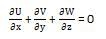
Continuity equation :
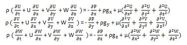
Momentum equations :
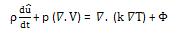
Energy equation :
Dimensionless Numbers :
Few important dimensionless numbers often encountered in multiphase flows study are as follows :
Reynolds number (Re) : It is the ratio of inertial force to viscous force, mathematically given by :

Peclet number (Pe) : It is the ratio of convective transport to molecular transport of energy or mass, given by :

Prandtl number (Pr) : It is the ratio of momentum diffusivity to thermal diffusivity, given as :

Schmidt number (Sc) : It is the ratio of momentum diffusivity to mass diffusivity, given by :

Nusselt number (Nu) : It is the ratio of total transfer to molecular transfer of energy represented as :

Stanton number (St) : It is the ratio of interface transport to bulk transport given as :
Weber number (We) : It is the ratio of inertial to surface forces represented as :

Multiphase flows – Modelling approaches :
- Eulerian specification : It focuses on specific locations in the space through which the fluid flows as time passes.
- Lagrangian specification : Here the observer follows an individual fluid parcel as it moves through space and time. Equations are composed by using this fundamental concept.
The modelling equations are composed keeping in mind the Eulerian and Lagrangian framework, we model the continuous phase by Eulerian method and depending upon the complexity of the flow we consider if the dispersed/ secondary phase can be modelled by Eulerian or Lagrangian framework. Multiphase flow can be modelled mainly by three different approaches listed below.
- Eulerian – Lagrangian Approach : Utilises Eulerian framework for the continuous phase and Lagrangian framework for dispersed phases
- Eulerian – Eulerian Approach : Utilises Eulerian framework for both the phases
- Volume of Fluid Approach : Eulerian framework for both the phases with specialised interface treatment.
This can be explained in detail as follows.
Eulerian-Lagrangian approach :
Let us imagine a vast continuum represented by blue colour as the continuous phase in the figure shown below and small particle spheres as the dispersed/ secondary phase. The discrete particle or the secondary phase in its motion is affected by the continuous phase and at times also affects the motion of continuous phase. By Eulerian-Lagrangian (E-L) approach, it means that the Eulerian framework governing equation is used for the continuous phase and the dispersed phase trajectories are solved using Lagrangian framework.
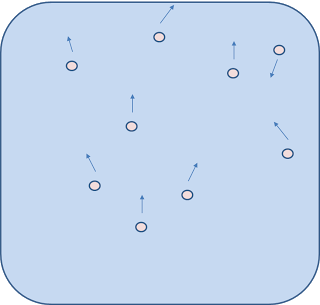
As they coexist there is a interface coupling between continuous and the dispersed phase i.e. as the dispersed phase particles moves in the continuous phase, due to drag, lift and various other forces there is exchange of momentum and energy between the two. This exchange takes place through coupling that can be one-way or two-way i.e the continuous phase can influence the dispersed phase flow or even the dispersed phase can influence the flow of continuous phase. The exchange of momentum and energy exists between the fluid (continuous phase) and the particle (dispersed phase) and is considered while modelling using the E-L framework.
The trajectories of the dispersed phase particles are solved not using the conventional Navier-Stoke’s equation but the equations of motions i.e. the Lagrangian framework. The E-L approach is however valid for simulating dispersed multiphase flows containing a low (<10%) volume fraction of dispersed phase. For higher volume fractions of dispersed phase one may necessarily have to use Eulerian-Eulerian approach.
e.g. gas-liquid flow in bubble column reactors
Eulerian-Eulerian approach :
In Eulerian-Eulerian (E-E) approach both the dispersed particle phase and continuous fluid phase are solved using the governing equations i.e. the Eulerian approach. The Lagrangian framework is not applied for dispersed phase. This can be explained using the figure given below that shows the distribution of continuous phase fluid (blue) and the dispersed phase particles (pink spheres).
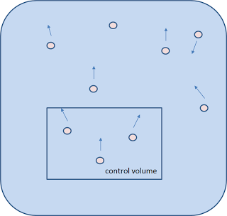
Here the control volume is used to define phase velocities i.e. both the phases are modelled using the Eulerian framework of governing equations and solved within the defined control volume to obtain the phase velocities. The volume fractions of both the phases are also solved at these control volumes. As explained earlier there is an exchange of momentum and energy between the two phases this two-way coupling is solved using volume average equations for the dispersed phase. The E-E approach is valid for denser (>10%) volume fractions of dispersed phase.
e.g. fluidized bed reactors, bubble column reactors, multiphase stirred reactors, etc.
Volume of Fluid approach :
The volume of fluid method is particularly applicable for stratified or separated flows where the dispersed phase is well separated from the continuous phase with a distinct interface, figure below. Here, a single set of governing equation is solved for both phases using combined mixture properties. The mixture properties are obtained by using the volume fraction of each phase. The weighted mixture properties i.e. density, viscosity, specific heat etc. are of the mixture and not of the individual phase.
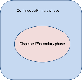
To obtain the location or position of the interface the volumetric forces are modelled using the interface tracking techniques. e.g. interfacial phenomena like wall adhesion, surface tension, etc.
The Author
{module [317]}