Understanding CFD Simulation Process with Examples
Having already explained the background & evolution of Computational Fluid Dynamics (CFD) in the earlier blog Introduction to CFD, let us now try to understand the CFD simulation process with a few examples."CFD is the science of predicting fluid flow, heat transfer, mass transfer, chemical reactions, and related phenomena by solving the mathematical equations which govern these processes using numerical methods"
It provides a qualitative and quantitative prediction of fluid flows by means of :
- Mathematical modeling (partial differential equations)
- Numerical methods (discretization and solution techniques)
- Software tools (solvers, pre- and post-processing utilities)
Simulation Process :
To understand the simulation process and the steps involved in it let us consider an example of a flow through a pipe bend. The figure below gives series of the steps that would be involved in its analysis. For a fluid flow through a pipe bend we have the geometry built up, segregated into smaller fragments/ segments, called a mesh. With this mesh we actually define our probe-points where we want the analysis to be done. We then define the boundary conditions to get a unique solution solving it with a computer. The results obtained gives us a lot of data along these probe points that are then post-processed with visualization tools to analyse the results.
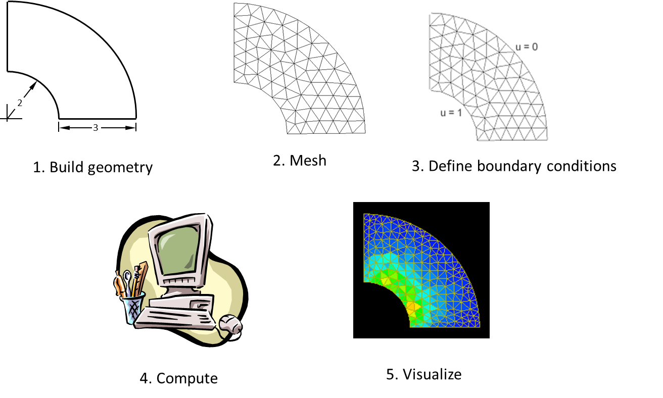 Thus CFD process in overall is a 3 step procedure :
- Pre Processing : This step consist of defining a geometry to define our domain of interest. The domain of interest is then divided into segments, called as mesh generation step and the problem is set-up defining the boundary conditions. Gridgen, CFD-GEOM, or ANSYS Workbench Environment & Modules, ANSYS ICEM CFD, TGrid etc., are some of the popular pre-processing softwares.
- Solver : Once the problem is set-up defining the boundary conditions we solve it with the software on the computer, (can also be done by hand-calculations, but would take long time). We have different popular commercial softwares available for this like Star-CD and Star CCM+ (CD-Adapco), FLUENT and CFX (ANSYS, Inc), GASP (Aerosoft, Inc), CFD++ (Metacomp Technologies) etc. Also there are free to use softwares like OpenFOAM, CFL3D, Typhon, OVERFLOW, Wind-US etc, all with different capabilities. These softwares are capable of solving the equations at every probe-point defined during the mesh generation step and also we can include additional models as required by the physics. The numerical methods are also defined at the this stage and we solve the whole problem.
- Post-processing : Once we get the results as values at our probe points we analyse them by means of color plots, contour plots, appropriate graphical representations & can generate reports. Tecplot 360, EnSight, FieldView, ParaView, ANSYS CFD-Post etc., are some of the popular post processing softwares.
How CFD Works ?
Now let us try to analyze a real life problem, with 2 examples discussed below.
1. Test Case: Fin-Tube Heat Exchanger
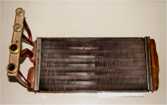
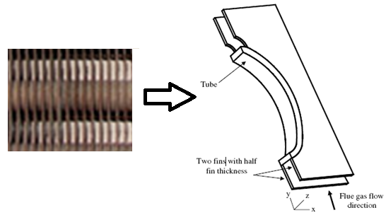 Domain of Interest: Area between two fins
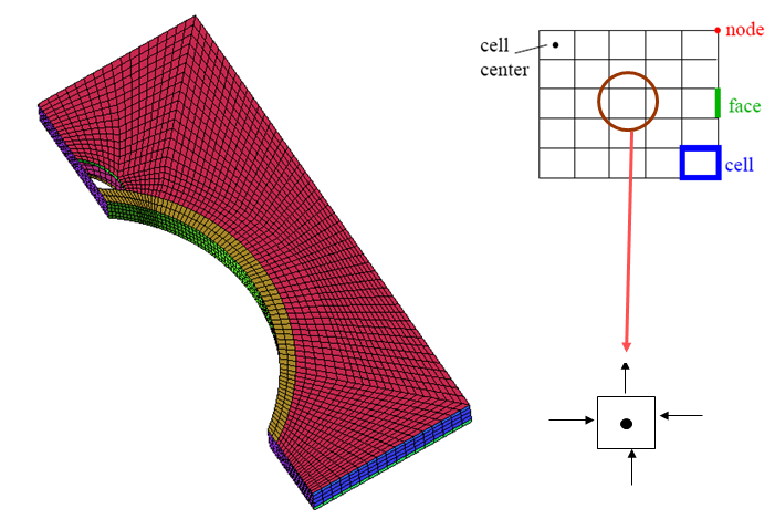
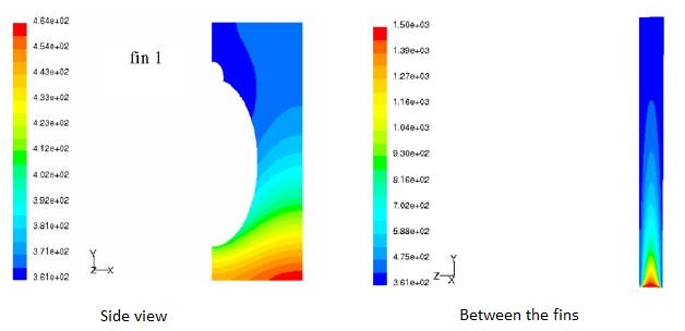
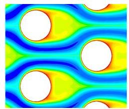
Temperature contours
2. Water flow over a tube bankConsider the analysis of a cascade of tubes placed inside a domain across which a fluid (water) is flowing. The objective here is to compute average pressure drop and heat transfer per tube row. So it is a physical system in which we have a complicated setup of several cascade of tubes. To start with, we shall not proceed to solve the real problem but would try to simplify it taking a section for analysis, set-up the problem, first gain confidence over it and then if the computational resources are available and if time permits, proceed to implement on the real problem.
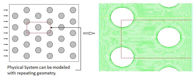
Geometry simplification
Assumptions
- flow is two-dimensional, laminar, incompressible
- flow approaching tube bank is steady with a known velocity
- body forces due to gravity are negligible
- flow is translationally periodic (i.e. geometry repeats itself)
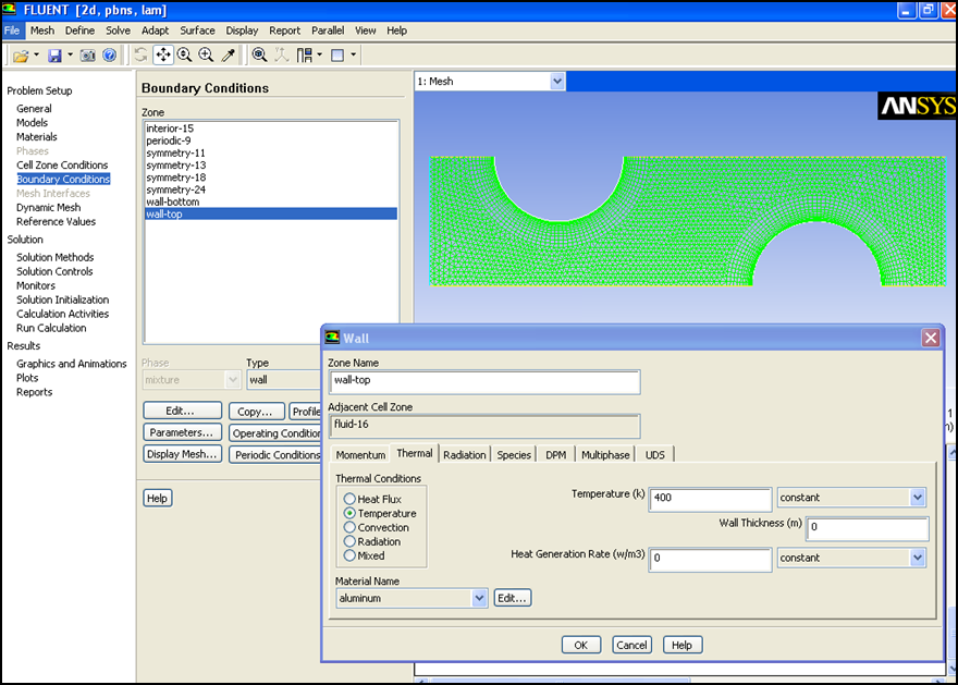
As can be seen from the discretized geometry above, we have a fine mesh size at near the wall of the tubes and coarser at the other regions, so as to resolve the boundary layer flow at these regions. We have a whole system being modeled as we set up the problem on a software for example, Fluent as in figure below. In the solver we import the mesh, select the appropriate solver methodology, define operating conditions (no-slip, Qw or Tw at walls), initialize and iterate to get a converged solution.
The Author
{module [317]}