Evaluate Solar Load using Computational Fluid Dynamics (CFD)
The article is about a popular model available in ANSYS FLUENT, the solar load model (SLM). Here we will try to understand the simple overview of SLM and also have a demo video of a test case created using for setting up the SLM. To understand its significance it would be interesting to understand the physics happening when we say solar loading.
Basically solar load is nothing but including the effect of energy transfer from the Sun's surface to the earth's surface, and as it takes place through vacuum, it's a radiation phenomena.
Heating due to incident solar rays is a very common but an important phenomenon. As we all know,enormous amount of energy is radiated from the Sun to planet earth. One of the common observation is that during day time the temperature rises and falls again at night as sun is not present in the horizon. Due to the increase in temperature (during day-time) majority of flows occur in our planet, for example wind starts blowing due to heating of some area locally,which indirectly affect many other phenomena. Apart from this simple example there are many such examples that make solar loading effects an important branch within CFD for research purpose, like heating of building walls which makes it necessary to analyze them and provide proper insulation within the building for human comfort (HVAC studies). In short, it is a very important in industrial research and optimization studies.
Understanding Solar Loading :
It is the amount of energy radiated to the object under study from sun rays. This energy varies primarily with the orientation of sun in the horizon. Cloud cover plays a crucial role in the solar loading of the earth bound objects.
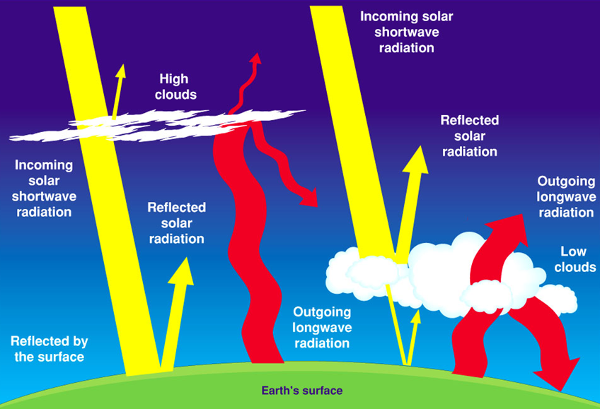
(Image source: www.ecoedility.it)
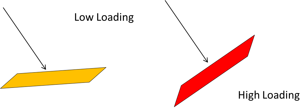
Variation of solar loading with incident angles
Let us first understand few of the terms related to solar radiation :
Now Let us understand few terms related to Solar Loading Model in Fluent
1. Sunshine Factor : It accounts for the cloud covering the sky at a given time and location under study. so it is basically percentage of cloud cover which range from 0 to 1 where 0 means completely covered with cloud and 1 means no cloud. The cloud cover basically reduces the sunlight from sun.
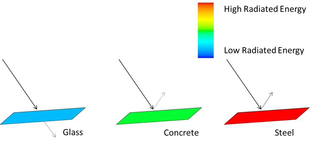
2. Ground Reflectivity : As the name indicates it includes the contribution of the reflected solar radiation from the ground. So in the SLM, higher the ground reflectivity higher is the solar radiation value and it is added into the diffuse solar radiation input.
Exploring the model :
You will find SLM window under the radiation model. It has a very simple and a learn-as-you-use type of interface
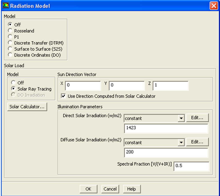
Solar loading model window in ANSYS FLUENT
Test Case :
- Latitude : 18.9647° N, 72.8258° E
- Time Zone : +5.5
- Month : June
- Date : 1st
- Time : 15:30 hrs
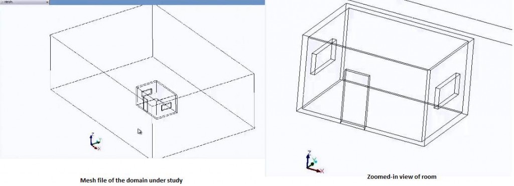
CAD model of room for study
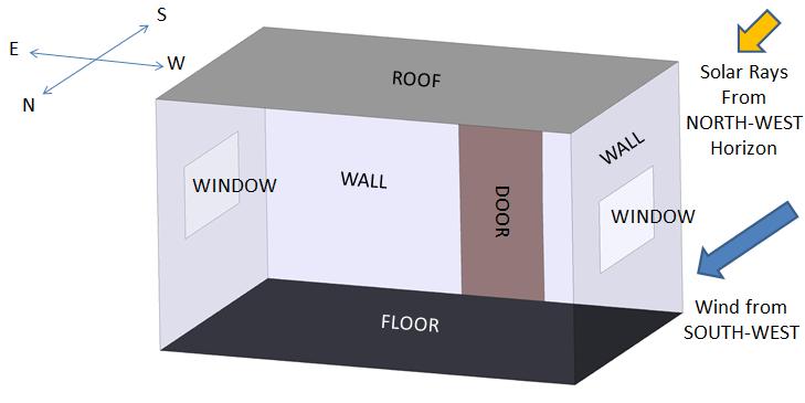
Geometry :
The below images show the CAD geometry of the room with its surrounding. In the geometry we have the air domain which contains a single room on which we will be studying the solar loading effect. Also we have the ground and inside domain where we have room with its thickness modeled having two windows and one door. In this case we will let air to enter the room and exit from the windows.
Problem setup :
The following steps are included in the problem setup :
- Turn ON gravity with correct orientation
- Activate solar load model setup, under radiation tab.
- Give appropriate settings within solar load model using the sun calculator, instead of manually providing it.
- In the text window, the values of the direction vector and the direct normal solar irradiation in [W/m2] is displayed.
- Setting up rest of the case and going for Initialization.
The point to be noted here is whenever we initialize a SLM details for a case, we have to start FLUENT in serial mode and not in parallel mode as parallel mode initialization of SLM in FLUENT is not possible. After initialization in the text window we can see the amount of solar loading being added to each and every wall of the room. Now as the heat loading is directly being added onto each wall, we can see the contours of loading at that very instance before the simulation process has started.
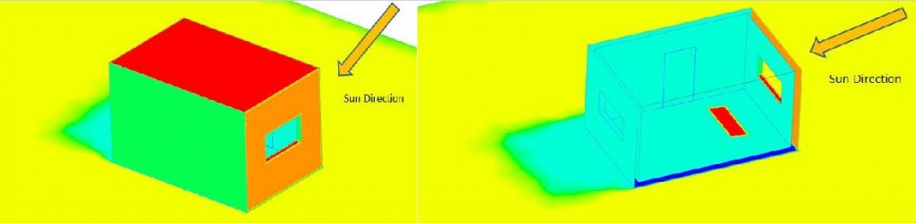
Solar heat flux contours
From above figure we can see that the shadow zone is clearly visible and the loading is nicely distributed on perpendicular as well as on almost parallel surfaces. You may observe that the shadow zone isn't having zero loading, but do have some heat radiated, this loading is because of the reflected rays. Also one can clearly notice that the walls in the shadow zones are of the same loading i.e. of same contour levels, both for inner and outer walls. This is better understood when one goes through the working of the Solar load model in Fluent.
Analysis :
Analysis begin by first checking the fluxes, then checking total mass flow rate for inlets and outlets, to see if it is completely balanced, i.e., the solution is converged. Later visualize the qualitative results starting with contours of temperature. In the following picture, flow direction is from right to left. The temperature contours plotted here is of the central cross-section passing through the room.
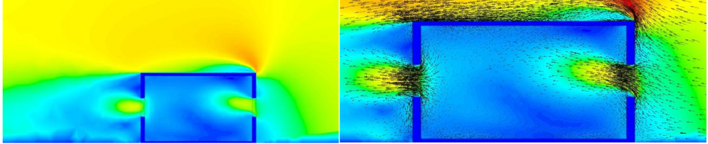
Temperature contours of the room
We have ambient temperature at inlet and it is growing inside the room due to solar loading. Another interesting thing to be noted is the wall conduction. In the zoomed-out view (right figure) we can see how heat is carried out by air. Now lets view the velocity reports at the central plane, here we can see the velocity decreases as we approach the room and velocity rises while it passes through the windows.
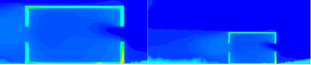
Velocity contours of air in the room
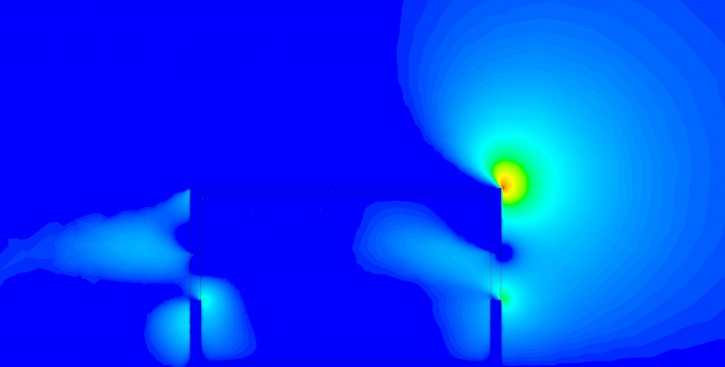
Z-direction (vertical) velocity contour
Looking at Z-direction (vertical) velocity contour on the central cross-sectional plane, we see, in the regions not colored with dark blue, velocities are in the positive vertical direction i.e. air is going up at those places. This indicates that once air enters the room from the window, it tends to rise because of natural convection. Now the outer yellow colored zone is basically the flow path that tends to rise above the room's roof while approaching the room. Now lets have a look at the flow path in and around the room colored by temperature on the left and velocity on the right(blue - low, red - high).
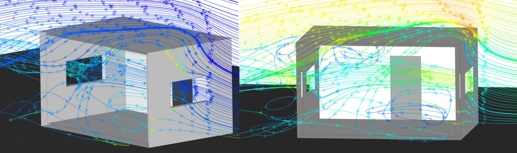
Pathlines in and around the room
In the left picture you can see that air enters at ambient temperature and leaves the room at an higher temperature. Thus with the SLM we can simulate the effects of solar heating and the convective flow currents produced with an ease. Below video shows the demonstration of the solar load modeling using ANSYS FLUENT software.
Software Demo :
|
{modal index.php/en/?option=com_content&view=article&id=114}
 {/modal} {/modal}
{modal index.php/en/?option=com_content&view=article&id=114}
 {/modal} {/modal} |
References :
1. ANSYS FLUENT user guide
The Author
{module [319]}