CFD Modeling for Turbomachinery using MRF Model
Having already gone through our blog series of CFD modeling of turbomachinery, wherein we discussed about the CAD Repair and Grid Generation we shall now explore the different solver models available in a commercial software package. CFD modeling of flows within systems containing moving components (e.g. turbomachines) are performed by resorting to moving reference frames (MRF). There are a number of both generalized and specialized commercial softwares available that apply moving reference frames for both translating and rotating systems. MRF approach finds application in a wide range of systems like turbomachinery, mixing equipment, electric motors and generators, rotating passages & land and air vehicle motions. In the current blog we shall try to understand applying MRF model for turbomachinery explained with the help of a simple test case.
The MRF approach however requires a special treatment as it has to accord with the modeling and analysis of various existing complex rotating system having components like a stator, rotor in single or multistage. Certainly all the parts attached to the rotating shaft are as well rotating with a certain angular velocity relative to the machine axis, whereas the stationary parts like the stator, casing, inlet(s), exit(s) etc., are devoid of any motion. Such flows for a stationary observer appears unsteady (around the moving parts) though apparently its a steady state case while when viewed by an observer posted on the rotor appears steady flow. For unsteady (transient) state flow problems the position of the observer hardly matters and is unsteady. Hence what remains important point is the synergy of information between the stationary frame and the moving reference frame.
For solving turbomachinery problems using CFD there exists specific and special models to be applied, and one of the models being popular in use is the Moving Reference Frame model. In MRF model a moving reference frame permits an unsteady problem (with respect to the absolute reference frame) to become steady in respect to the moving reference frame. In other words the complete rotor domain is assumed to be rotating at the same angular velocity of the rotor. Since basically all turbomachinery flows are unsteady in nature, the moving reference frame model approach makes simpler to solve these problems in CFD. It makes it easier to specify appropriate boundary conditions requiring less time and computational efforts and therefore is the preferred choice in industrial practices over rest of the models.
When a moving reference frame is activated, the equations of motion are modified to incorporate the additional acceleration terms i.e., Coriolis and centripetal acceleration terms which occur due to the transformation from the stationary to the moving reference frame. By solving these equations in a steady-state manner, the flow around the moving parts can be modeled.
Few of the models available in commercial softwares like ANSYS FLUENT are :
- Single Reference Frame model (SRF)
- Multiple Reference Frame model (MRF)
- Mixing Plane Model (MPM)
- Sliding Mesh Model
For simple problems, it may be possible to refer the entire computational domain to a single moving reference frame. This is known as the single reference frame (or SRF) approach. The use of the SRF approach is possible, provided the geometry meets certain requirements. For more complex geometries like a centrifugal pump with volute casing, it may not be possible to use a single reference frame. In such cases, the domain is differentiated into multiple cells zones, with well-defined interfaces between the zones. The manner in which the interfaces are treated leads to two approximate, steady-state modeling methods for this class of problem: the multiple reference frame (or MRF) approach, and the mixing plane approach. If unsteady interaction between the stationary and moving parts is important, Sliding Mesh approach is employed to capture the transient behavior of the flow.
Before getting into the details of the individual models let us get familiar with few terms.
- Surface of revolution : A surface of revolution is a surface generated by rotating a two-dimensional curve about an axis. e.g. cylindrical, spherical, conical.
- Interface : A boundary across which two independent domains meet and across which information is exchanged. The interface separating rotating and stationary domain must be a surface of revolution with respect to axis of rotation of the rotating zone. The interface should be placed such that there are no stationary components which are not a surface of revolution, inside the rotating zone.
The modified equations for moving reference frame are as given below:
Conservation of mass:
{tex} \frac{\partial(\rho)}{\partial t} + \nabla \cdot \rho \vec {v_r} = 0 {/tex}
Conservation of momentum :
{tex} \frac{\partial(\rho \vec v_r)}{\partial t} + \nabla \cdot (\rho {\vec v_r} {\vec v_r}) + \rho (2\vec {w} \times \vec {v_r} + \vec {w} \times \vec {w} \times \vec{r})= - \nabla p + \nabla (\bar {\bar {\tau_r}}) + \vec{F} {/tex}
{tex} \vec v_r = \vec v - \vec u_r {/tex}
{tex} \vec u_r = \vec{\omega} \times \vec{r} {/tex}
where {tex}\vec{v_r} {/tex} and {tex} \vec{v} {/tex} is the absolute velocity, {tex}\vec{u_r} {/tex} is the whirl velocity.
The momentum equation contains two additional acceleration terms i.e. the Coriolis acceleration: {tex} 2\vec{\omega} \times \vec{v_{r}}{/tex} acceleration terms: the Coriolis acceleration and the centripetal acceleration: {tex} \vec{\omega} \times \vec{\omega} \times \vec{r} {/tex}.
Single Reference of Frame (SRF) model:
Many problems permit the entire computational domain to be referred to as a single rotating reference frame (hence the name SRF modeling). In such cases, the equations given above are solved in all fluid cell zones. Steady-state solutions are possible in SRF models provided suitable boundary conditions are prescribed. But the wall boundaries must meet certain requirements, as mentioned below:
- The wall which is moving with the reference frame may assume any shape.
- Boundaries which are stationary should be the surface of revolution about axis of rotation.
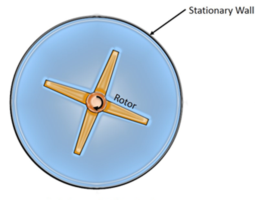
An example where SRF approach can be applied is shown above. In the example, the domain contains a rotor which is moving at certain angular velocity and a stationary wall. In this case the problem can be solved using SRF approach, since no stationary walls are present inside the domain and the outer stationary wall is surface of revolution and meets the above criteria. But when the problem involves multiple rotating parts or stationary components (like guide vanes in turbines) that are not the surface of revolution, the SRF modelling approach fails. Thus a different approach has to be adopted to solve such kind of problems by breaking the domain into stationary zone and rotating zone with interface separating them. Based on the manner in which interface is treated two approaches are defined namely :
1. Multiple Rotating Reference Frames
- Multiple Reference Frame model (MRF)
- Mixing Plane Model (MPM)
2. Sliding Mesh Model (SMM)
Here we shall discuss more about only the MRF model.
Multiple Reference Frame (MRF) model:
The MRF model is the simplest of the two approaches for multiple zones. It is a steady-state approximation in which individual cell zones move at different rotational and/or translational speeds. The flow in each moving cell zone is solved using the moving reference frame equations. If the zone is stationary {tex}(\omega = 0){/tex}, the stationary equations are used i.e., moving reference frame equations are solved in rotational zone and stationary equations are solved in stationary zone and the information is exchanged at the interface. The properties of the flow at the interface between the stationary and rotating zones is directly translated in MRF. In MRF approach there is no relative motion between moving zone with respect to the adjacent zone, the grid is fixed for computation. This is analogous to freezing the motion of the moving part in a specific position and observing the instantaneous flow field with the rotor in that position and hence, the MRF is often referred to as the "frozen rotor approach."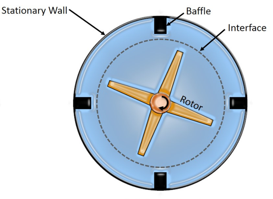 An example that illustrates the MRF approach is shown with an above (image). In the image apart from the rotor and stationary walls there are stationary baffles present inside the fluid zone. Thus an interface is defined which is a surface of revolution about the rotor axis to distinguish between stationary and rotating zone. MRF model should be used when the flow is not complicated and if the interaction between rotor and stator in a turbine stage is weak. With a MRF simulation rotating wakes, secondary flows, leading edge pressure increases etc.will always stay in exactly the same positions. This makes the simulation very dependent on exactly how the rotors and the stators are positioned. Usually MRF model is used to calculate flow field that can be used as initial condition for sliding mesh calculation.
Test case:
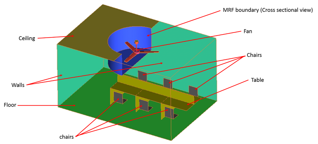
Below shows a test case on simulation of fan in a room using MRF model. The objective of the test case is to distinguish the two zones i.e. rotating and stationary with an interface to solve using MRF model and to visualize the flow circulation around the objects inside the room. The CAD model of the room with ceiling fan MRF boundary and other details is shown below:
- Objective: To determine whether the velocity of air at seating area lies in the human comfort range
- Fan rotation speed: 200 rpm
- Fan blades: 3, each separated by an angle of 120∘
- Fan blade twist angle : 8∘
The contours of velocity in both horizontal and vertical plane in the middle and velocity vector is shown below.
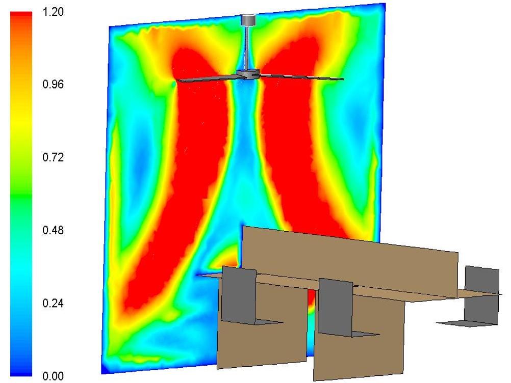
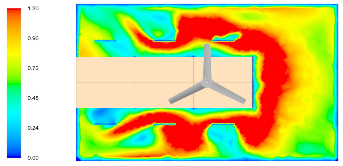
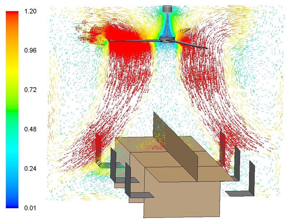
From the velocity contour and vector in the middle plane, the convection current can be seen clearly. As seen in the images above it becomes clear that the velocity of air behind the blades is small or almost nil, but increases as it crosses the moving blades in the downward direction. Also from the velocity contour in the middle plane it can be seen that the air is circulating around chairs causing the desired comfort.
|
{modal index.php/en/?option=com_content&view=article&id=135}
 {/modal} {/modal}
{modal index.php/en/?option=com_content&view=article&id=135}
 {/modal} {/modal} |
Reference:
- FLUENT user guide- modelling flows with rotating reference frames.
- esi CFD FAQ- http://www.esi-cfd.com/faq/index.php?action=artikel&cat=4&id=19&artlang=en
- http://en.wikipedia.org/wiki/Rotating_reference_frame
- http://www.beilke-cfd.de/rotflow1.pdf
The Author
{module [317]}